Completing this analysis required data on several variables. First, I required data on house prices, structural characteristics, neighborhood characteristics, and demographic characteristics. Following that, I would need to join this data to a measure of the tree canopy present in any given neighborhood.
The American Community Survey (ACS) met much of the first data need. In their 5-year assessment, last administered in 2011, the ACS measured median property values, numbers of rooms in structures, travel times to work, and characteristics of residents including age, education, and race & ethnicity. Their data is recorded at the block-group level. While this does not provide as high a level of resolution as individual households would, it was the smallest unit of measurement not considered proprietary information (and therefore the smallest unit of measurement available to me).
The block-group-level resolution has other important implications, however. The most important is the way in which it addresses the possible external benefits of tree canopy, where individual households may benefit from the “spillover effects” of tree canopy that is not on their own property, but in proximity to it. By using the block group as the base unit of analysis, the area surrounding each individual house is already included. One other implication to note is that my individual data points are already averaged values, however, which is what allows for statistics such as a maximum household size of 3.63—this is the maximum average household size for a block group.
Data on Portland’s tree canopy were not readily available in a directly analyzable format. As best as I can tell, no one has yet published a data set that details what proportion of each of Portland’s block groups is covered by tree canopy. As this measurement represented a cornerstone of my analysis, however, I deemed it essential to acquire, and I used this opportunity to produce the data for myself.
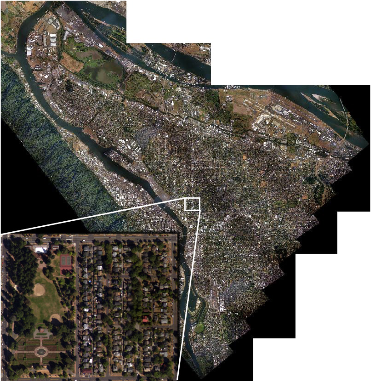
Doing so involved analysis of the United States Geologic Survey (USGS)’s 2012 Aerial Orthoimagery of Portland. This is a set of 2500-square-meter quadrants of high-resolution aerial imaging, adjusted for perspective distortion so as to be the same true-area representation of space that a map would be. I compiled 51 of these orthophotos into a single, massive raster image of Portland-from-above using Geographic Information Systems—ArcGIS, in my case. The resulting raster image is shown below, which represents a true-area, high-resolution, imagery data set which approximates Portland city limits.
The next step involved classification of the raster by land cover type, so as to be able to determine what proportion of any given area was covered by tree canopy. Having deemed manual classification infeasible (though not for lack of trying, as those who read my posts know), I set to work with a Spatial Analytics tool called Maximum Likelihood Classification. This method of analysis uses a signature file of classified training samples to fit each pixel of a raster file to the category in which it most likely belongs. It considers the RGB value of each pixel as well as the pixels around it, and chooses the most likely category of the signature file based on the patterns of pixels in the raster image. By creating a sufficiently representative signature file, I was able to classify Portland’s land cover to an extent that, while not perfect, provided an accurate enough representation to enable comparison of different areas based on the amount of canopy each contained. The results are shown below.
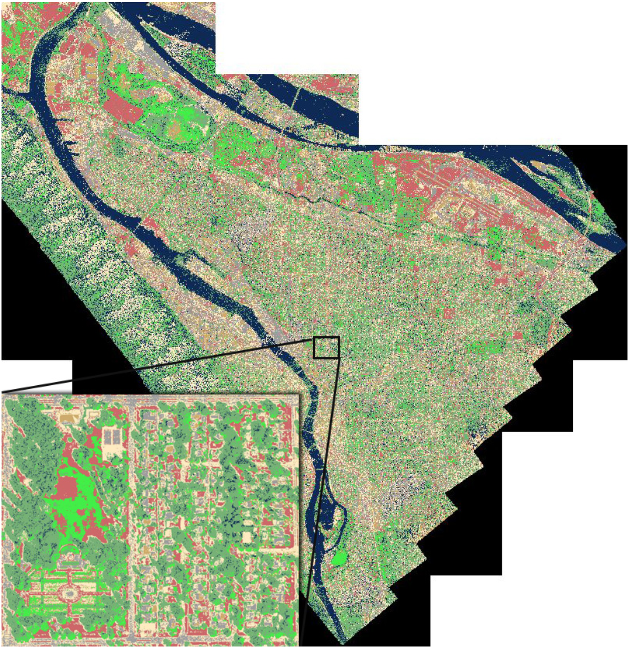
Having now produced a massive raster file of Portland classified by land cover type, it remained to me to separate these data by block group, quantify them, and join them to the remaining data. I accomplished this with a Zonal Histogram, which separates data into defined zones (in my case, block groups) and counts the number of pixels in each value class. I represented each block group by the number of tree canopy pixels it contained divided by the total number of pixels it contained, giving me a proportion of each block group which was covered by tree canopy. I then joined these data to my remaining data, including another GIS task of sorting crime incidents into block groups to generate a local crime count. At the end of this process, I had a data set suitable for regression analysis.