Interestingly, though I researched and learned how to use these classifiers, I never actually took the time to investigate how they actually worked or where they came from. I am sort of struggling to decide how much detail to go into. There are a lot of parts of these classifiers and details of pre-processing that I actually don’t understand at all. So I think for a general audience, I can really only go so far that I can accurately explain the algorithms.
The Support Vector Machine (SVM) is a type of supervised machine learning, which analyzes data for classification and is also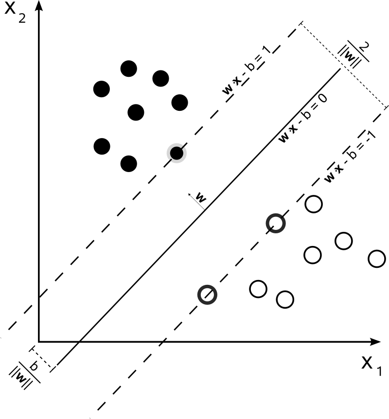 used in regression analysis. While the concepts and pieces of SVM have been around since the 20th century, the application for pattern recognition was introduced in the 1990’s and then continually tuned and refined (Suykens 1). The specifics of the algorithm are complex and varied, but very simply, the algorithm constructs optimal hyperplanes between the data points to separate them into different classifications. This is very difficult to visualize in higher dimensions, but you can see a two dimensional representation in the figure to the right.
For the classifiers, we leaned heavily on the findings of Zhou et al. who compare the methodologies of some of the primary cloud classification papers. Unlike our images, the images they use are more similar to images taken by standard cameras, meaning they are portions of the sky with minimal distortion. Since the instrument captures the sky with a mosaic of images, the sun can be more easily avoided. Interestingly, in terms of the linguistic method of classification, “Liu et al. (2011) argued that the criteria developed by the WMO (1975) for classifying different cloud types is unsuitable for automatic cloud classification” (Zhou et al. 85). This is definitely evident in many cloud classification papers which sometimes group cloud classes like cumuliform or waveform, although there is no consensus on this convention. More standard to cloud classification is the practice of leaving out rare cloud classes because of a lack of a robust training data. Zhou et al found that, in terms of the effectiveness of the classifier, the SVM performed the best. The K Nearest Neighbor (KNN) with just the single closest neighbor was the next best. Then came KNN with 3 and 5 and then neural networks coming in last. For our classification, we decided not to explore neural networks since other cloud classification papers using it did not perform as well. However, for comparison we also used KNN with various numbers of neighbors.
The KNN classifier to much easier to explain and implement since it classifies based just on distance. When a new image’s statistics are fed into KNN, a distance from the images statistics in the training set is calculated. If the nearest neighbor is set to one, the image is classified with the class of the closest image in the training set. If the nearest neighbor is set to a number greater than one, the image is classified with the majority class. A number of reputable cloud classification papers use KNN including Peura et al. 1996; Singh and Glennen 2005; Isosalo et al. 2007; Heinle et al. 2010. even though as wikipedia puts is, k-NN is “among the simplest machine learning algorithms.”
Zhou et al. also evaluate the effectiveness of the type of color preprocessing. Interestingly, Zhou has R/B as the worst performing color space. This is the one we primarily use. However, we also calculate statistics on the intensity image (which performed mid range in the color space comparison). Since the TSI images are so different from Zhou’s images, there are also some operations which would be impractical for our images, like dividing the image into blocks with similar texture. We don’t have the luxury of a relatively flat rectangle of sky. However, this rectangle is not representative of the whole sky like the TSI is. It is hard to say whether the differences between their results and ours are due to the different type of image or the differences in preprocessing.