Background:
In order to understand and utilize SPSS, a Statistics Datafile application, we decided to explore the correlation between the healthy average life expectancy and the NET agricultural output of any given country. The United Nations Environment Programme (UNEP) Environmental Data Explorer contains databases with more than 500 variables ranging from national, subregional, regional, as well as global statistics. Information is accessible on topics spanning freshwater, population, forests, emissions, climate, disasters, health, and GDP. These statistics can be downloaded in various formats including maps, graphs, and data tables. The UNEP databases allowed us to gather the data that we were interested in, synthesize it, and plug it into the SPSS to better analyze the correlation.
The Healthy Average Life Expectancy, HALE, “is based on life expectancy, but includes an adjustment for time spent in poor health. This indicator measures the equivalent number of years in full health that a newborn child can expect to live based on the current mortality and prevalence distribution of health states in the population” (HALE metadata). In other words, the overall health of a population is studied in order to create an approximation of what can be expected for the health of future generations.
The Net Production Index – Agriculture “show[s] the relative level of the aggregate volume of agricultural production for each year in comparison with the base period 2004-2006. They are based on the sum of price-weighted quantities of different agricultural commodities produced after deductions of quantities used as seed and feed weighted in a similar manner” (Net Production Index – Agriculture metadata). All crops, except for fodder crops, and livestock products stemming from each country are included. The index is obtained by dividing a year’s aggregate by the average aggregate between 1999 and 2001.
The question we attempted to answer was, how is the healthy average life expectancy affected by the increase or decrease of a country’s agricultural output. Because the NET agricultural output is measured in percentage compared to previous years out of 100 (ie. 110 is equal to a 10% increase), and the HALE is measured by expected years, we were able to see if increasing agricultural production affects local lifestyles in a definitive way. We predicted that these changes to come from pesticide and herbicide use, economic changes, and many other environmental and social shifts that follow agricultural production.
Procedure:
Utilizing the UNEP Environmental Data Explorer, we drew the available statistical data for HALE and percent change in total agricultural output (PCTAO) for over 250 countries. We navigated the raw data using Microsoft Excel and deleted those countries with no data, which were identifiable by the “-9999” in the data cell. Using Excel functions, we found the percent rank for each country based on its HALE and PCTAO. Using the HALE percent rank of each country, we were able to group each country into quintiles 1-5. To obtain a random sample of the total country population (greater than 250), we assigned each country a randomized number and chose the 90 highest numbers along with the corresponding countries.
By importing the 90 countries with their HALE and PCTAO values into the SPSS, we calculated the the difference in means and tested for any possible correlations. Our results, while from the sample, were used as a way to infer conclusions about the larger population.
Results:
| N | Mean | Std. Dev. | 2-tailed Sig. (P-value) | |
| Quartile 1 | 19yrs | 65yrs | 6yrs | 0 |
| Quartile 5 | 24yrs | 52yrs | 11yrs | 0 |
Fig 1.
Mean Differential: For quintiles 1 and 5, there were 19 and 24 countries, respectively. Mean HALEs were approximately 65 years and 52 years, respectively, resulting in a difference of means of 14 years. Standard deviations were 6 years and 11 years, respectively.
| Pearson Correlation (r-value) | Sig. (2-tailed) | N |
| -0.47 | 0.0 | 90 |
Fig. 2
Correlation: The correlation was calculated using an N of 90 sample countries. As shown in Fig. 2, The probability value (P-Value, two-tailed significance value) was 0.0. and the r-value (Pearson Correlation) was recorded at -0.47.
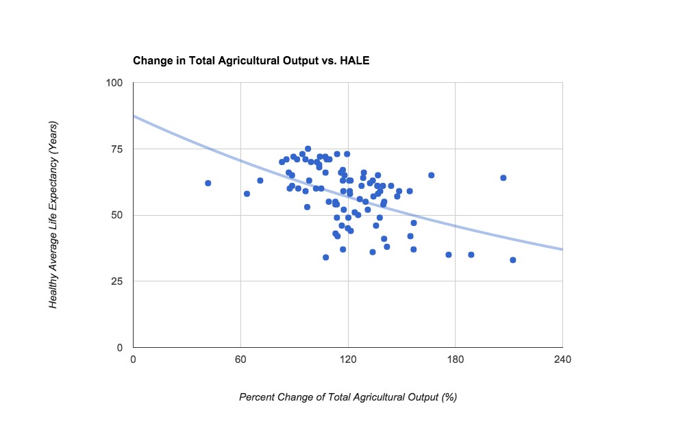
Fig. 3
Discussion:
When analyzing the synthesized data from SPSS, the information that was most applicable was the mean, standard deviation, p-value, and r-value. The mean of quartile 1 is a 65 year HALE, while the quartile 5 is 52 years. This means that as the agricultural production increases, the HALE decreases: a negative relationship. This correlation is supported by the recorded Pearson Correlation of -0.47; furthermore, the relationship can be deemed significant because the p-value was found to be less than 0.05 (recorded at 0.0). Thus, we are able to reject the null hypothesis that HALE would remain constant even as PCTAO changes.
In interpreting this negative relationship between HALE and PCTAO, we drew real world scenarios that would match our outcomes, namely, that involving quinoa and quinoa farmers.Quinoa has recently spiked in popularity internationally (Raynolds et al. 2007), and this has fueled an increased output of quinoa production in those countries from which the crop originates. The surplus quinoa has hiked the consumer prices in western countries, creating a cyclical relationship in which consumers create demand, while producers drive down local living conditions in order to keep up with the increasing demand (Jacobsen 2011). In this example, PCTAO of quinoa increases while HALE is lowered due to decreased living standards.
Works Cited:
Raynolds, Laura T. et al. Fair Trade: The Challenges of Transforming Globalization. Routledge, 2007: 180-181. Print.
Jacobsen, S.-E. “The Situation for Quinoa and Its Production in Southern Bolivia: From Economic Success to Environmental Disaster.” Journal of Agronomy and Crop Science 197.5 (2011): 390–399. Wiley Online Library. Web.