Team Members: Jesse Simpson, Perri Pond, and Nick Pankratz
Background
In this lab, we analyzed the statistical relationships between our environmental variable from last week’s lab and three variables which potentially play a role in driving global disparities of per capita carbon dioxide emissions, across the 25 nations Lewis and Clark has study-abroad programs in. We chose to analyze gross capital formation (as a percent of GDP), infant mortality rate, and percent share urbanized. We selected these variables as they each relate to national economic development, which we consider central to per capita carbon emissions, yet relate to “development” in perhaps a more novel way than a simple GDP per capita analysis. We focused on two core statistical values in this exploration: the p-value and r-value. The p-value is the probability that the null hypothesis (that there is no relationship between the variables) is true, while the r value is a measure of the correlation between two variables. The p-value ranges between 0 and 1, with 0 representing no possibility of the null hypothesis being true, and 1 representing a 100% probability that the null hypothesis holds. The R value, meanwhile, ranges between -1 and 1, with -1 representing a completely linear negative correlation, with no deviation, 1 representing a completely linear positive correlation, and 0 representing no linear correlation in the data. In order for a relationship to be statistically significant, we need to have a p-value of ≤ 0.05, which represents a 95% confidence interval; for a relationship to be substantially significant, we need an R value of ≥|0.2|.
The three statistical analyses which we will conduct over the course of this lab are a simple difference in means test, a zero-order correlation, and a linear regression. The difference in means test is an analysis of data predicated on the creation of two distinct groups from the independent variable; after demarcating the two groups, one analyzes the mean of the dependent variable of both groups, and conducts a T-test to find the significance of the difference in means. A zero-order correlation, meanwhile, looks at how each of the variables are related to one another linearly, on the basis of their R and p values. It does not, however, correct for interactions among multiple variables, as a linear regression does. Through the magic of computers, a linear regression quickly accounts for overlap in the independent variables in determining the dependent variable, and churns out a standardized coefficient and p value for each of the independent variables in concert with each other.
Procedure
We began this lab by finding the descriptive statistics of our data. First, we sorted all the countries based on our driving variable and then determined a cutoff point that distinguished between the lower and higher categories. Then, we moved our data into a SPSS dataset and ran a descriptive analysis for our driver variable. We collected the mean, median, mode, standard deviation and skewness. Next, we began our inferential statistics analysis by running a difference of means test for each of our test variables. We split each variable’s data set into two roughly equal groups for this analysis. We each ran an Independent Sample T Test, using .05 for our alpha (required p value). From this test we found the mean per capita carbon dioxide emissions of the two country groups of each of the three driver variables, and the significance of the difference in means. Next, we ran a zero-order correlation between all of our variables to find the degree of correlation between each of our driver variables and per capita carbon emissions, as quantified by R and p values. Our last step was conducting a linear regression to assess the causality of our driver variables, in relation to each other. We maintained a 95% confidence interval and included the standardized beta. From our results we were able to analyze the strongest statistical relations between our environmental or dependent variable and our independent variables.
Results
Difference of Mean
[table]
,Infant Mortality,Urban Population,Capital Formation
Mean (Group 1),2.5,2.7,4.7
Mean (Group 2),8.5,7.9,7.0
p-value,0.001,0.004,0.242
[/table]
In our difference of mean analysis, we found a statistically significant relationship (p ≤0.05) between both infant mortality and urban population share and per capita carbon dioxide emissions, with a dramatically less significant, though existent, relationship between capital formation and per capita carbon dioxide emissions.
Note that Group 1 and Group 2 consist of different countries for each statistic, with group 1 for infant mortality consisting of the 13 countries with an infant mortality above 6 deaths per 1,000 live births, group 1 for urban population consisting of the 11 countries with less than 66% of their populace living in urban areas, and group 1 for capital formation composed of the 11 countries with more than 20% of their GDP consisting of capital formation. In each case, group 1 emits less carbon dioxide per capita than group 2. This preliminary analysis points to a potential strongly negative relationship between infant mortality and per capita carbon emissions, a potential strongly positive relationship between urbanization and per capita carbon emissions, and a weakly negative relationship between capital formation and carbon dioxide emissions per capita.
Zero-Order Correlation
[table]
, ,CO2 per capita,Capital Formation,Infant Mortality,Urban Population
CO2 per capita,R value,—,-0.165,-0.704,0.641
,p-value, ,0.431,0,0.001
Capital Formation,R value,-0.165,—,0.183,-0.191
,p-value,0.431, ,0.383,0.360
Infant Mortality,R value,-0.704,0.183,—,-0.791
,p-value,0,0.383, ,0
Urban Population,R value,0.641,-0.191,-0.791,—
,p-value,0.001,0.360,0,
[/table]
From our zero-order correlation analysis, we found significant relationships between infant mortality and per capita CO2 emissions (R value of -0.704 and a p-value of 0), urban population and per capita CO2 emissions (R value of 0.641 and a p-value of 0.001), and between infant mortality and urban population (R value of -0.791 and a p-value of 0). From this analysis, it is clear that there is some kind of relationship between these three variables, as the correlations exceed even a 99% confidence interval. Capital formation has essentially no relationship to any of the other three variables analyzed here, with no correlation between capital formation and another variable clearing our thresholds of an R value ≥|0.2| and a p-value less than 0.05.
Linear Regression Analysis
[table]
,Infant Mortality, Urban Population, Capital Formation
R value,-0.524,0.221,-0.027
p-value,0.047,0.384,0.864
[/table]
By conducting a linear regression, we found that infant mortality was substantially and statistically related in a causative way with per capita carbon dioxide emissions, with an R value of -0.524 and a p-value of 0.047. With the linear regression, however, urban population became remarkably less significant of a driving variable, with an R value of only 0.221 and a p-value of 0.384. Gross capital formation was neither substantially nor statistically significant with an R value of -.027 and a p-value of 0.864. Additionally, the adjusted R squard coefficient generated by this regression indicates that our variables account for 44% of the variation in per capita carbon dioxide emissions, after adjusting for overlap between the independent variables
Discussion
Each of our analyses point to the significance of the negative relationship between infant mortality and per capita carbon dioxide emissions, with an adjusted coefficient of -0.524 and a p-value of 0.047 in the linear regression analysis; infant mortality was the only variable which cleared our confidence interval in this final analysis. The results of our linear regression cannot be taken at face value, however; this fact becomes apparent when one vocalizes its most direct interpretation—that decreased infant mortality is causative of increased per capita CO2 emissions, and can account for nearly half of the global disparity in per capita carbon emissions. Keeping in mind that we are using a per capita measure of CO2, which controls for whatever increased population results from 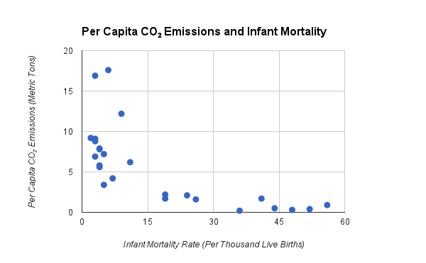 decreased infant mortality, we are thus led to the argument that infant mortality is merelya proxy for the societal and economic conditions of nations, with these disparities in development accounting for a large portion of the global disparity in carbon footprints. It would be interesting to repeat this analysis with per capita GDP, to measure if a more direct economic indicator is more or less statistically causative than infant mortality.
The interpretation of infant mortality as merely an approximation of carbon-intensive economic development is further supported by how the urban population variable behaved over the course of our statistical analyses. Urban population was statistically and substantively correlated with per capita CO2 emissions, yet this relationship disappeared under the rigors of the linear regression, suggesting that this variable overlaps with infant mortality in terms of its causative powers. The strong negative correlation between urban population and infant mortality is also supportive of this interpretation; in our results, we saw that the negative relationship between urbanization and infant mortality was almost exactly as strong as that between carbon dioxide per capita and infant mortality.
One surprising piece of data we found is that there is little to no correlation between gross capital formation and the carbon dioxide emissions per capita. We had hypothesized that there would be a relationship between the two, as capital formation comprises the most visible and physical aspects of economic development—altering land and building infrastructure, buildings and factories. It seems intuitive that countries engaged in a greater share of this frequently polluting form of development would also have greater per capita carbon emissions. Yet we found no such trend. In every analysis conducted, gross capital formation was neither substantially significant nor statistically significant. Digging into the data, we found that both developed and underdeveloped nations tended to have low values of gross capital formation. For example, the United Kingdom has a gross capital formation share of 15% and Swaziland has a capital formation share of 9%. These values are dwarfed by those of rapidly industrializing, yet still poor, nations. China topped the list with a 49% share, and was followed by Tanzania, Morocco, India, and Ecuador. This is reflected to some degree in our quantitative data, as capital formation was not correlated with infant mortality or percent urbanized. Perhaps capital formation would arise as a more significant variable in determining CO2 emissions over an extended temporal scale, as nations investing more in infrastructure and the means of production could see greater carbon-intensive economic growth. When examining a single year, however, the percent of GDP devoted to capital expansion has no statistical impact on per capita carbon dioxide emissions