Over this past week, I’ve delved deep into my regression analysis of the property values around the Orange Line. It’s been an intensely iterative process, as I’ve moved back and forth between several different ways of setting up a regression model while churning through the seemingly endless mounds of previous transit-related hedonic studies, slowly building an understanding of the relevant terminology and methodologies. The foundation of my model is the hedonic model—examining the relationship between prices over time with respect to the network distance to Orange Line stations, controlling for structural and other locational attributes. There are many choices to make with regard to each of these terms, choices whose implications and motivations I only roughly understand at the moment. The dependent variable, price, can be expressed directly or as its natural logarithm. Taking the log of price both unskews the distribution and turns the term into an expression of the percentage change in price. The focus independent variable of the study, network distance from rail, can be similarly logged, creating a log-log model that expresses the relationship between distance and price as an elasticity—easily interpreted as the percent change in price given a percent change in distance. This log-log model allows for the proximity effects of transit to be viewed as an inverse exponential curve, with price effects most dramatic near the station. As one approaches the station, a given absolute change in distance will become a larger and larger percentage change, with this percentage change being the relevant factor for determining the percentage change in price.
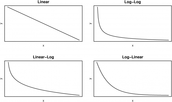
Illustration of Different Functional Forms of Regressions
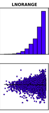 It’s also worth noting that many studies use distance band specifications, examining the relationship between price and transit proximity within vs outside a given radius. I find this rather arbitrary and think some sort of logistic transformation better captures the reality of diminishing utility of transit as distances increase. In the regressions I performed this week, however, the log-log form appears to be somewhat problematic, introducing a high degree of heteroskedasticity (an increase in errors as the variable increases). The plot shown at the right is the regressed relationship between the natural log of station distance (horizontal axis) and the natural log of price (vertical axis)—it’s essentially the perfect image of heteroskedasticity, which is apparently quite problematic in statistical analysis. Over the coming week or two I will need to address this issue, via some kind of different model specification.
The statistical choices compound further when we consider the controlling independent structural or locational variables. My present data set includes a limited number of structural variables, owing to the paucity of the public dataset—simply the age of the structure, the square footage of the building, and the square footage of the lot. This leaves out many of the structural variables commonly used in hedonic models, like the number of bedrooms, bathrooms, and stories, the presence of a garage, deck/patio, or other amenities, rated building quality, architectural style, and heating/cooling systems. The use of these variables in hedonic regression seems basically dependent on the availability of data, with more fields considered better. For the three structural variables I do have, there is additionally the option to transform the variables by using their natural log or squared value. Yan et al. (2013), for instance, take the natural log of building area and use an age-squared variable along with age (to capture the tendency for homes to acquire some historic value at a certain point). For my present and interim regression model, I took the natural log of building and lot square footage and used both the age and age-squared variables.
The subjectivities of statistical analysis compound even further when we move to the locational attributes. I began with a focus on other proximity attributes, like the distance to heavy rail, highways, parks, rivers, commercial and industrial zoning, grocery stores, community centers, and the Orange line itself; the percentage of streets with sidewalks; the average age of structures within a quarter of a mile; and a measure of slope (the sum feet of 10 foot contour lines contained within a tenth of mile of the property). These attributes were driven by the availability of data and hypothesized potential amenity or disamenity effects. After reading Yan et al. (2013), who simply used dummy variables for each block group that the home sales are in to control for locational variation, I became interested in this apparently straightforward (though time-consuming) method. The resulting model, however, was slightly less explanatory than the previous model (Adj. R-squared=.52), displayed roughly the same amount of residual clustering (as measured with Moran’s I), and showed no significance for either of the Orange Line variables. Including some block group demographic data (median household income, percent of residents with a bachelor’s degree, and percent non-white), a dummy variable for being located in the Portland city limits, alongside the slope (FT_CONTOUR), mean year of surrounding structures (MEANYR_STR), the log distance to downtown, and a temporal index variable (LOGSCIND—the S&P Case-Shiller index for the Portland metro area for each month, achieved the highest explanatory power of models tested. The results of this regression are below.
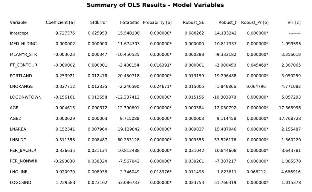
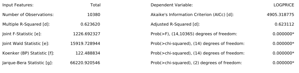
The most relevant variables for my thesis are LNORANGE (natural log of network distance to stations) and LNOLINE (natural log of straight-line distance to the line itself). In this particular specification, they both lie right on the edge of statistical significance—the main p-value for both is <.05 but the Koenker Statistic indicates that there is significant heteroskedasticity, meaning that the Robust Probability must be used. The coefficients accord with theory, indicating a .027% decrease in price with a 1% increase in walking distance to the station and a .021% increase in price with a 1% increase in distance from the line itself (the line runs largely in an industrial right-of-way). This would mean that, holding all else (including the distance to the line) equal, a property .25 miles from the station would be worth 13.5% more than one 1.5 miles away. Viewed in space, with estimated values transformed from logs back into dollars, this model’s estimated values and standard residuals are below:


Considering the dramatic diversity of transit land value uplift hedonic models extant in the literature, as surveyed by Higgins (2016), it seems that there is no singular “right choice” with regard to model specification. Nevertheless, with reference to Armstrong and Rodriguez (2006), it has also come to my attention that I need to more systematically evaluate the “spatial lag” of these variables, in conjunction with whatever treatment of the heteroskedasticity I find.
Leave a Reply