Over this last week, I re-consulted the hedonic literature to gather new ideas for model specification and variables, reading through papers until the Greek letters and statistical language started to make sense. I also decided to do some more formalized data validation. I spot checked properties exhibiting high standard residuals in my regression analysis through Zillow, Redfin, Trulia, and the source County Assessor’s site, to ascertain if any of the provided fields were outdated or misspecified. The outdated errors mostly come in the form of properties which have been recently demolished, which was readily assessed using PortlandMaps sales and permit data and/or Google Streetview. If I was able to find a new figure of the house square footage, I inputed that figure; if not, I deleted the field. The mispecification errors arose through the somewhat odd data management necessitated by PortlandMaps’s taxlot-based data. In Clackamas County in particular, there are many undeveloped taxlot slivers that are obviously sold as part of an associated house, yet recorded as separate transactions for the same price, though only for the characteristics embodied by the small, undeveloped lot. For taxlot sliver errors, I removed the sliver sale from the dataset and added its lot square footage to the associated home sale.
I made a large move forward in tackling the issues of spatial autocorrelation that had been visibly plaguing my model by using spatial fixed effects—namely, dummy variables of the official neighborhood that each property is within. Drawing on Duncan (2007), I have chosen to rely heavily on specifications of neighborhoods to control for neighborhood effects with no good quantitative measure. Previously, I had attempted to control for neighborhood variables through block group dummy variables, following Yan’s (2013) model. Not only was this very cumbersome, but the specification seems likely to soak up any of the locational effects of rail. Instead, I used the boundaries of neighborhood associations, which provide a larger proxy for locational effects. I spatially joined the neighborhood association shapefile to the sales points and manually created the series of dummy variables based on the assigned neighborhood. These variables were highly significant and returning coefficients in line with expectations of the housing market, representing the estimate premium or discount assigned to neighborhoods relative to the Richmond neighborhood. Including the neighborhood dummy variables increased R-squared by about 6-8% and greatly reduced the spatial autocorrelation of residuals.
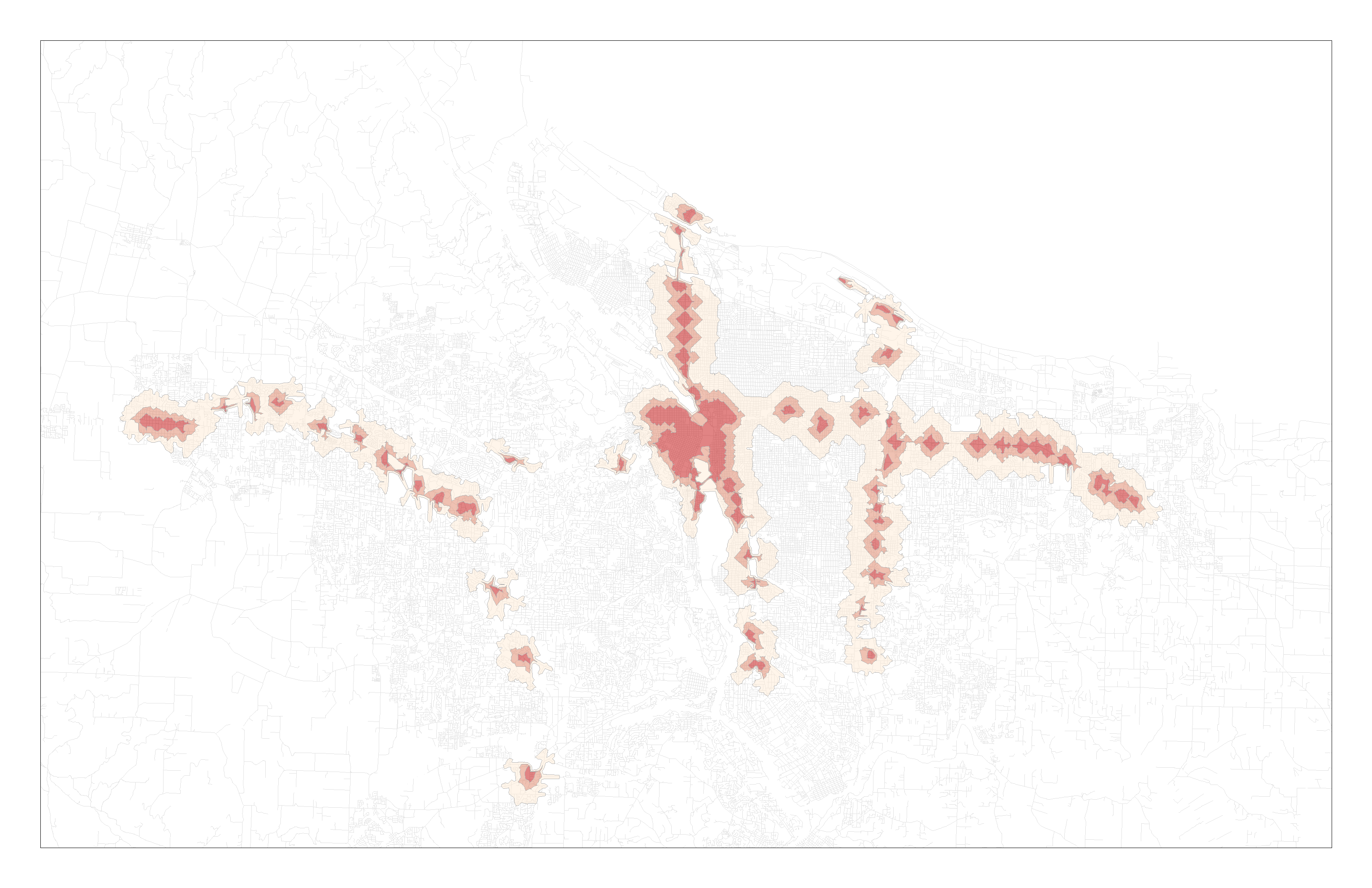
I further delimited the bounds of my study to 1.25 miles in network distance. Since this equates to roughly a 25 minute walk, it seems unreasonable that a station premium would persist past that point and most hedonic analysis find price effects, if any, in the range of a quarter mile to one mile (Higgins and Kanaroglou 2016). Leaving a larger than necessary study area will tend to increase the errors involved in estimating the coefficients of variables while perhaps. This was prompted first by realizing that I was including large parts of the Southwest Hills in my analysis—up to 2 miles walking distance from the nearest station. There’s little reason to believe that such locations are valuing the addition of the Orange Line for providing one-hour total travel time access to Milwaukie.
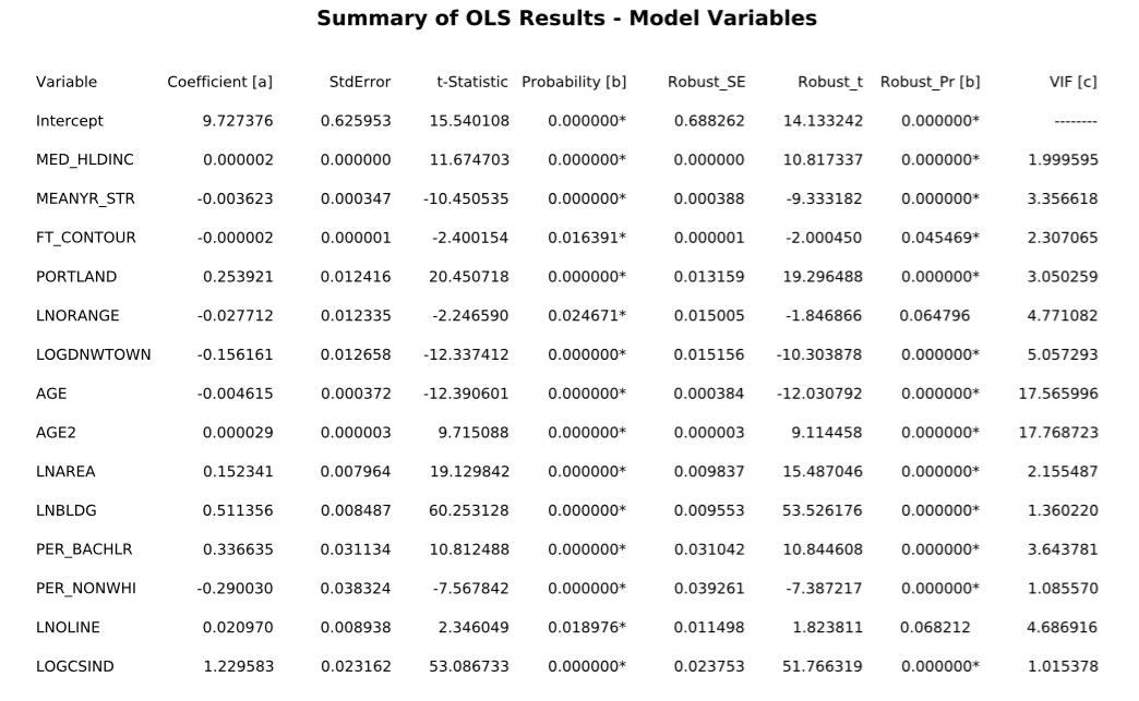
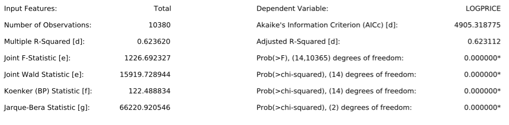
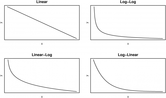
I have essential settled on the level-log specification for my model. Leaving the independent variable untransformed is attractive for theoretic and practical considerations. Taking the logarithm of the price means that every dependent variable’s effect is interpreted as yielding a percentage change, and thus the effects would be greater for more expensive homes. Also, interpreting logarithms is difficult, with the transformation back into regular prices apparently a big statistical no-no. Nevertheless, I would expect to see a curved function of some sort, as the change in the value of proximity would seem to increase more with increased proximity—the change in value from half a mile to a quarter of a mile is surely greater than than of going from 1.25 to one, representing a much larger percentage decrease in time taken to access transit. Alongside this continuous variable, I also ran models with dummy variables created for quarter mile distance bands for cross-verification purposes. In terms of other variable modification, I changed the variable measuring the median age of surrounding homes (quarter mile buffer) into a measure of the percentage of surrounding homes that were built before 1940. This variable was more significant in the model than a simple linear age and more closely approximates the effect I had in mind when I created the age variable—the increased price associated with being around historic homes in prewar neighborhoods. I also created a variable for whether a home is attached, based on the property code description. My model suggests that this brings a ~$30,000-$45,000 discount. I also changed the posited disamenity rail variable from the continuous distance variable to dummy distance bands. The continuous variables were quite odd to interpret with the station proximity variable, as any resultant price effects are the effects of increasing your proximity to the station while holding the distance to the line constant, which only happens in the case of disconnected street grids or by moving parallel to the line. The resultant coefficients were also much larger than anticipated while biasing the estimate of the station proximity upward. The hedonic model results obtained are posted below, with the White standard errors shown due to significant heteroskedasticity remaining. I think I need this to be my final specification, considering that we’re running out of time in the semester and I still need to do significant work on individual station models.


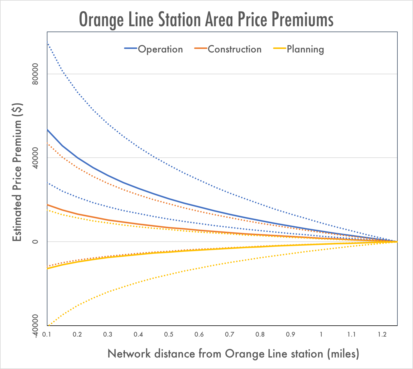
Overall, the results show the progressive development of a light rail premium from planning to operation. Distance to stations (lnOLSta) goes from being insignificantly positive to insignificantly negative to significantly negative from planning to construction to operation, resulting in a price premium equal to $230 per 1% decrease in the distance to the station, or $63,000 for properties within a quarter mile and $30,000 between a quarter and three-quarters of a mile. One can derive a dollar estimate of the price premium resulting the continuous logarithm coefficient. Though this value is technically calculated within the model as the expected change in price given a one-log change from the mean log-distance, the price premium from light rail can be derived from this estimate by assuming that the premium at 1.25 miles is zero. From this, we can create a table of the estimated percentage change in price from 1.25mi by multiplying the percentage change in distance by the coefficient. 95% confidence intervals were created by multiplying the standard error by the relevant t score and then adding this margin of error to the coefficient.
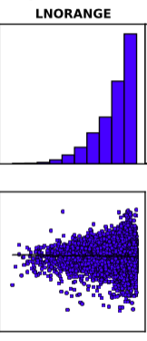 It’s also worth noting that many studies use distance band specifications, examining the relationship between price and transit proximity within vs outside a given radius. I find this rather arbitrary and think some sort of logistic transformation better captures the reality of diminishing utility of transit as distances increase. In the regressions I performed this week, however, the log-log form appears to be somewhat problematic, introducing a high degree of heteroskedasticity (an increase in errors as the variable increases). The plot shown at the right is the regressed relationship between the natural log of station distance (horizontal axis) and the natural log of price (vertical axis)—it’s essentially the perfect image of heteroskedasticity, which is apparently quite problematic in statistical analysis. Over the coming week or two I will need to address this issue, via some kind of different model specification.